Python處理PDF與CDF實例
在拿到數據后,最需要做的工作之一就是查看一下自己的數據分布情況。而針對數據的分布,又包括pdf和cdf兩類。
下面介紹使用python生成pdf的方法:
使用matplotlib的畫圖接口hist(),直接畫出pdf分布;
使用numpy的數據處理函數histogram(),可以生成pdf分布數據,方便進行后續的數據處理,比如進一步生成cdf;
使用seaborn的distplot(),好處是可以進行pdf分布的擬合,查看自己數據的分布類型;
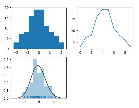
上圖所示為采用3種算法生成的pdf圖。下面是源代碼。
from scipy import statsimport matplotlib.pyplot as pltimport numpy as npimport seaborn as snsarr = np.random.normal(size=100)# plot histogramplt.subplot(221)plt.hist(arr)# obtain histogram dataplt.subplot(222)hist, bin_edges = np.histogram(arr)plt.plot(hist)# fit histogram curveplt.subplot(223)sns.distplot(arr, kde=False, fit=stats.gamma, rug=True)plt.show()
下面介紹使用python生成cdf的方法:
使用numpy的數據處理函數histogram(),生成pdf分布數據,進一步生成cdf;
使用seaborn的cumfreq(),直接畫出cdf;
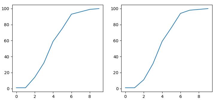
上圖所示為采用2種算法生成的cdf圖。下面是源代碼。
from scipy import statsimport matplotlib.pyplot as pltimport numpy as npimport seaborn as snsarr = np.random.normal(size=100)plt.subplot(121)hist, bin_edges = np.histogram(arr)cdf = np.cumsum(hist)plt.plot(cdf)plt.subplot(122)cdf = stats.cumfreq(arr)plt.plot(cdf[0])plt.show()
在更多時候,需要把pdf和cdf放在一起,可以更好的顯示數據分布。這個實現需要把pdf和cdf分別進行歸一化。
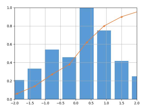
上圖所示為歸一化的pdf和cdf。下面是源代碼。
from scipy import statsimport matplotlib.pyplot as pltimport numpy as npimport seaborn as snsarr = np.random.normal(size=100)hist, bin_edges = np.histogram(arr)width = (bin_edges[1] - bin_edges[0]) * 0.8plt.bar(bin_edges[1:], hist/max(hist), width=width, color=’#5B9BD5’)cdf = np.cumsum(hist/sum(hist))plt.plot(bin_edges[1:], cdf, ’-*’, color=’#ED7D31’)plt.xlim([-2, 2])plt.ylim([0, 1])plt.grid()plt.show()
以上這篇Python處理PDF與CDF實例就是小編分享給大家的全部內容了,希望能給大家一個參考,也希望大家多多支持好吧啦網。
相關文章:

 網公網安備
網公網安備